If you have not done the Buttons exercise from Exercise 2, we suggest that you start by finishing it.
The aim of exercise three is:
Most of the exercise concerns control of the ball and beam process.
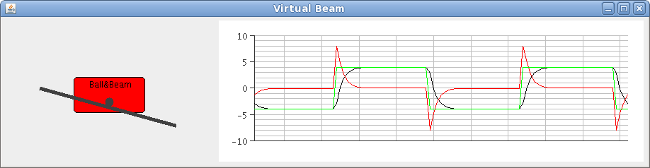
Instead of using the real process you will use a virtual, simulated ball and beam process. A Swing-based GUI to the controllers is available. A reference signal generator class is also provided. During Laboratory 1 the real ball and beam process will be used.
So far you have implemented periodic tasks only using sleep, i.e., as
  long h = ...; // Sampling interval
  try {
    while (!Thread.interrupted()) {
      periodicActivity();
      Thread.sleep(h);
    }
  } catch (InterruptedException x) {
    // Requested to stop
  }
where h is the desired period in milliseconds. The problem with this approach is that it does not take the execution time of the periodic activity into account. The execution time includes the actual execution, which may be time-varying due to, e.g., caches, data-dependent operations, and the time when the thread is suspended by other threads.
A better, although far from perfect, way to implement periodic threads is the following
  long h = ...; // Sampling interval
  long duration;
  long t = System.currentTimeMillis();
  try {
    while (!Thread.interrupted()) {
      periodicActivity();
      t = t + h;
      duration = t - System.currentTimeMillis();
      if (duration > 0) {
        Thread.sleep(duration);
      }
    }
  } catch (InterruptedException x) {
    // Requested to stop
  }
In the following you should use this approach as soon as you implement periodic controller tasks.
In this exercise your task is to implement a PI controller and use it to control the angle of the ball and beam process, i.e., without any ball. The controller should be split up in two parts: the class PI which only contains the basic PI algorithm and the class BeamRegul which implements the control of the beam process with the use of a PI controller.
For the implementation you should use two predefined classes: PIParameters containing the parameters of a PI controller and PIGUI that implements a graphical user interface for the PI through which you can change controller parameters.
The PI controller should be implemented in the class PI as a monitor, i.e., a passive object with only synchronized methods: PI code skeleton
The PIGUI class provides a Swing JFrame through which you can type in new values for the PI-parameters. If an invalid entry is made, e.g. a non-number, the change is ignored. In order to make it possible to change several parameters at the same time, a change does not take place until the Apply button has been pressed. The integratorOn is set to false if Ti is set to 0.0. The PI parameters in PIGUI get their initial values set through the constructor of PIGUI, which has the signature:
public PIGUI(PI PIReference, PIParameters initialPar, String name);
public class PI {
  private PIParameters p;

  private double I; // Integrator state

  private double v; // Desired control signal
  private double e; // Current control error

  //Constructor
  public PI(String name) {
	  PIParameters p = new PIParameters();
	  p.Beta = 1.0;
	  p.H = 0.1;
	  p.integratorOn = false;
	  p.K = 1.0;
	  p.Ti = 0.0;
	  p.Tr = 10.0;
	  new PIGUI(this, p, name);
	  setParameters(p);

	  this.I = 0.0;
	  this.v = 0.0;
	  this.e = 0.0;
  }

  public synchronized double calculateOutput(double y, double yref) {
	  this.e = yref - y;
	  this.v = p.K * (p.Beta * yref - y) + I; // I is 0.0 if integratorOn is false
	  return this.v;
  }

  public synchronized void updateState(double u) {
	  if (p.integratorOn) {
		  I = I + (p.K * p.H / p.Ti) * e + (p.H / p.Tr) * (u - v);
	  } else {
		  I = 0.0;
	  }
  }

  public synchronized long getHMillis() {
  	return (long)(p.H * 1000.0);
  }

  public synchronized void setParameters(PIParameters newParameters) {
  	p = (PIParameters)newParameters.clone();
	if (!p.integratorOn) {
		I = 0.0;
	}
  }
}
BeamRegul is the controller thread that implements the control of the beam process through the use of the PI class. The class ReferenceGenerator provides the reference signal with the method
public synchronized double getRef();
The ReferenceGenerator generates a square-wave signal. It has a GUI through which the amplitude and period (in seconds) can be changed.
import SimEnvironment.*;

public class BeamRegul extends Thread {
	private ReferenceGenerator referenceGenerator;
	private PI controller;

	private AnalogSource analogIn;
	private AnalogSink analogOut;
	private AnalogSink analogRef;

	//Define min and max control output
	private double uMin = -10.0;
	private double uMax = 10.0;

	//Constructor
	public BeamRegul(ReferenceGenerator ref, Beam beam, int pri) {
		referenceGenerator = ref;
		controller = new PI("PI");
		analogIn = beam.getSource(0);
		analogOut = beam.getSink(0);
		analogRef = beam.getSink(1);
		setPriority(pri);
	}
	//Saturate output at limits
	private double limit(double u, double umin, double umax) {
		if (u < umin) {
			u = umin;
		} else if (u > umax) {
			u = umax;
		}
		return u;
	}

	public void run() {
		long t = System.currentTimeMillis();
		while (true) {
			// Read inputs
			double y = analogIn.get();
			double ref = referenceGenerator.getRef();

			synchronized (controller) { // To avoid parameter changes in between
				// Compute control signal
				double u = limit(controller.calculateOutput(y, ref), uMin, uMax);

				// Set output
				analogOut.set(u);

				// Update state
				controller.updateState(u);
			}
			analogRef.set(ref); // Only for the plotter animation

			t = t + controller.getHMillis();
			long duration = t - System.currentTimeMillis();
			if (duration > 0) {
				try {
					sleep(duration);
				} catch (InterruptedException e) {
					e.printStackTrace();
				}
			}
		}
	}
}
The class Beam is a simulated "virtual" ball and beam process without any ball. It shows a plotter and an animation of the process.
> javac -classpath .:virtualsimulator.jar *.java
NOTE: This exercise is a preparatory exercise that must be done in order to be allowed to do Laboratory 1. No solution is available.
The next task is to implement a controller for the entire Ball and Beam Process (with the Ball). More information about the model for this process is available in BallAndBeamModel.pdf. The control structure that you should use is a cascade controller. This structure is suitable when an intermediate process output is available, that lies between the process input and the process output that you want to control. In the ball and beam process we want to control the position of the ball. However, we also have access to the angle of the beam. In a cascade controller the intermediate process output is used to close an inner control loop, according to the Figure below:
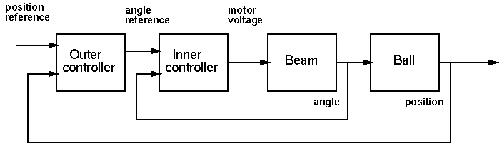
The output from the outer controller now becomes the reference for the inner controller. The advantages of a cascaded controller are that
When a cascade structure is used it is common to only have integral action in the outer loop. When we use cascaded control on the ball and beam process we use the same sampling interval for both controllers, and implement them in a single periodic thread. It is also quite common to use a faster sampling interval for the inner controller. When implementing the two loops in a single controller thread it is important to minimize the computational delay (control delay, latency) from the sampling of the position to the generation of the control signal.
Since the ball dynamics has negative gain, positive feedback is needed in the outer loop. The easiest way to achieve this is to use a negative K.
Suitable parameter ranges are:
  // Declarations
  private AnalogSource analogInAngle;
  private AnalogSource analogInPosition;
  private AnalogSink analogOut;
  private AnalogSink analogRef;

  // In Constructor
  analogInPosition = bb.getSource(0);
  analogInAngle = bb.getSource(1);
  analogOut = bb.getSink(0);
  analogRef = bb.getSink(1);
  >> K = 10;
  >> s = tf('s');
  >> Gbeam = 4.4 / s;
  >> Ginner = K*Gbeam / (1 + K*Gbeam);
  >> Gball = 7 / s^2; % assume negative controller gain
  >> nyquist(Ginner*Gball);
  >> margin(Ginner*Gball); % what are the stability margins?